Sensitivity Analysis

Setup

First, we will load the AEME and aemetools package:

library(AEME)
library(aemetools)

Create a folder for running the example calibration setup.

tmpdir <- "sa-test"
dir.create(tmpdir, showWarnings = FALSE)
aeme_dir <- system.file("extdata/lake/", package = "AEME")
# Copy files from package into tempdir
file.copy(aeme_dir, tmpdir, recursive = TRUE)
#> [1] TRUE
path <- file.path(tmpdir, "lake")

list.files(path, recursive = TRUE)
#> [1] "aeme.yaml"            "data/hypsograph.csv"  "data/inflow_FWMT.csv"
#> [4] "data/lake_obs.csv"    "data/meteo.csv"       "data/outflow.csv"    
#> [7] "data/water_level.csv" "model_controls.csv"

Build AEME ensemble

Using the AEME functions, we will build the AEME model setup. For this example, we will use the glm_aed model. The build_aeme function will

aeme <- yaml_to_aeme(path = path, "aeme.yaml")
model_controls <- AEME::get_model_controls()
inf_factor = c("dy_cd" = 1, "glm_aed" = 1, "gotm_wet" = 1)
outf_factor = c("dy_cd" = 1, "glm_aed" = 1, "gotm_wet" = 1)
model <- c("gotm_wet")
aeme <- build_aeme(path = path, aeme = aeme,
                       model = model, model_controls = model_controls,
                       inf_factor = inf_factor, ext_elev = 5,
                       use_bgc = TRUE)

Description of Sensitivity Analysis method

The sensitivity analysis method used here is based on the Sobol method and uses the sensobol package.

This package provides several functions to conduct variance-based uncertainty and sensitivity analysis, from the estimation of sensitivity indices to the visual representation of the results. It implements several state-of-the-art first and total-order estimators and allows the computation of up to fourth-order effects, as well as of the approximation error, in a swift and user-friendly way.

For more information on the method, see the sensobol package vignette.

Load parameters to be used for the sensitivity analysis

Parameters are loaded from the aemetools package within the aeme_parameters dataframe. The parameters are stored in a data frame with the following columns:

• model: The model name

• file: The file name of the model parameter file

• name: The parameter name

• value: The parameter value

• min: The minimum value of the parameter

• max: The maximum value of the parameter

Parameters to be used for the calibration. (man)

utils::data("aeme_parameters", package = "AEME")
param <- aeme_parameters |>
  dplyr::filter(file != "wdr")
param

model	file	name	value	min	max	module	group
glm_aed	glm3.nml	light/Kw	5.8e-01	0.100	5.52e+00	hydrodynamic	NA
glm_aed	met	MET_wndspd	1.0e+00	0.700	1.30e+00	hydrodynamic	NA
glm_aed	met	MET_radswd	1.0e+00	0.700	1.30e+00	hydrodynamic	NA
glm_aed	glm3.nml	mixing/coef_mix_conv	1.4e-01	0.100	2.00e-01	hydrodynamic	NA
glm_aed	glm3.nml	mixing/coef_wind_stir	2.1e-01	0.200	3.00e-01	hydrodynamic	NA
glm_aed	glm3.nml	mixing/coef_mix_shear	1.4e-01	0.100	2.00e-01	hydrodynamic	NA
glm_aed	glm3.nml	mixing/coef_mix_turb	5.6e-01	0.200	7.00e-01	hydrodynamic	NA
glm_aed	glm3.nml	mixing/coef_mix_hyp	7.4e-01	0.400	8.00e-01	hydrodynamic	NA
glm_aed	inf	inflow	1.0e+00	0.500	2.50e+00	hydrodynamic	NA
gotm_wet	gotm.yaml	turbulence/turb_param/k_min	6.0e-07	0.000	1.00e-05	hydrodynamic	NA
gotm_wet	gotm.yaml	light_extinction/A/constant_value	5.5e-01	0.395	6.59e-01	hydrodynamic	NA
gotm_wet	gotm.yaml	light_extinction/g1/constant_value	5.9e-01	0.440	7.40e-01	hydrodynamic	NA
gotm_wet	gotm.yaml	light_extinction/g2/constant_value	2.0e-01	0.050	2.70e+00	hydrodynamic	NA
gotm_wet	met	MET_wndspd	1.0e+00	0.700	1.30e+00	hydrodynamic	NA
gotm_wet	met	MET_radswd	1.0e+00	0.700	1.30e+00	hydrodynamic	NA
gotm_wet	inf	inflow	1.0e+00	0.500	2.50e+00	hydrodynamic	NA
dy_cd	cfg	light_extinction_coefficient/7	9.0e-01	0.100	1.40e+00	hydrodynamic	NA
dy_cd	dyresm3p1.par	vertical_mixing_coeff/15	2.0e+02	50.000	7.50e+02	hydrodynamic	NA
dy_cd	met	MET_wndspd	1.0e+00	0.700	1.30e+00	hydrodynamic	NA
dy_cd	met	MET_radswd	1.0e+00	0.700	1.30e+00	hydrodynamic	NA
dy_cd	inf	inflow	1.0e+00	0.500	2.50e+00	hydrodynamic	NA

Sensitivity analysis setup

Define fitness function

First, we will define a function for the sensitivity analysis function to use to calculate the sensitivity of the model. This function takes a dataframe as an argument. The dataframe contains the observed data (obs) and the modelled data (model). The function should return a single value.

Here we use the model mean.

# Function to calculate mean model output
fit <- function(df) {
  mean(df$model)
}

Different functions can be applied to different variables. For example, we can use the mean for water temperature and median for chloophyll-a.

# Function to calculate median model output
fit2 <- function(df) {
  median(df$model)
}

Then these would be combined into a named list of functions which will be passed to the sa_aeme function. They are named according to the target variable.

# Create list of functions
FUN_list <- list(HYD_temp = fit, PHY_tchla = fit2)

Define control parameters

Next, we will define the control parameters for the sensitivity analysis. The control parameters are generated using create_control and are then passed to the sa_aeme function. The control parameters for the sensitivity analysis are as follows:

?create_control

create_control

R Documentation

Create control list for calibration or sensitivity analysis

Arguments

method

The method to be used. It can be either "calib" for calibration or "sa" for sensitivity analysis.

...

Additional arguments to be passed to the function create_control. The arguments are different for calibration and sensitivity analysis. There are arguments which are common to both methods: file_type string; file type to write the output to. Options are c("csv", "db"). Defaults to "db". file_name string; file name to write the output to. Defaults to "results.db" if file_type is "db" and "simulation_metadata.csv" if file_type is "csv". file_dir string; directory to write the output to. Defaults to the directory "calib_sa" in the current working directory. If the directory does not exist, it will be created. na_value value to replace NA values with in observations. Defaults to 999. parallel boolean; run calibration in parallel. Default to TRUE ncore: The number of cores to use for the calibration. This is only used if parallel = TRUE. Default to parallel::detectCores() - 1. timeout: The maximum time in seconds to run the calibration. Default to Inf. If the calibration takes longer than the timeout, the calibration will stop and return the best parameter set found so far. For calibration, the arguments are: VTR Value to be reached. The optimization process will stop if either the maximum number of iterations itermax is reached or the best parameter vector bestmem has found a value fn(bestmem) <= VTR. Default to -Inf. NP number of population members. Defaults to NA; if the user does not change the value of NP from NA it is reset as 10 * sum(param$model == model). For many problems it is best to set NP to be at least 10 times the length of the parameter vector. itermax the maximum iteration (population generation) allowed. Default is 200. reltol relative convergence tolerance. The algorithm stops if it is unable to reduce the value by a factor of reltol * (abs(val) + reltol). Default = 0.07 cutoff: The quantile cutoff used to select the parents for the next generation. For example, if cutoff = 0.25, the best 25% of the population will be used as parents for the next generation. mutate fraction of population to undergo mutation (0-1). c_method character; the method to use for calibration. Options are "CMAES" and "LHC". Defaults to "CMAES". For sensitivity analysis, the arguments are: N: The initial sample size of the base sample matrix. vars_sim: A named list of output variables for sensitivity analysis. The name is user defined but each list must contain: var: The variable name to use for the sensitivity analysis. month: A vector of months to use for the sensitivity analysis. depth_range: A vector of length 2 with the minimum and maximum depth range to use for the sensitivity analysis.

Here is an example for examining surface temperature (surf_temp) in the months December to February, bottom temperature (bot_temp), (10 - 13 m) and also total chlorophyll-a (PHY_tchla) at the surface (0 - 2 m) during the summer period.

ctrl <- create_control(method = "sa", N = 2^4, ncore = 2, na_value = 999,
                       parallel = TRUE, file_name = "results.db",
                       vars_sim = list(
                         surf_temp = list(var = "HYD_temp",
                                          month = c(12, 1:2),
                                          depth_range = c(0, 2) 
                         ),
                         bot_temp = list(var = "HYD_temp",
                                         month = c(12, 1:2),
                                         depth_range = c(10, 13)
                         ),
                         surf_chla = list(var = "PHY_tchla",
                                          month = c(12, 1:2),
                                          depth_range = c(0, 2)
                         )
                       )
)

Run sensitivity analysis

Once we have defined the fitness function, control parameters and variables, we can run the sensitivity analysis. The sa_aeme function takes the following arguments:

?sa_aeme

sa_aeme

R Documentation

Run sensitivity analysis on AEME model parameters

Arguments

aeme	aeme; object.
path	filepath; where input files are located relative to 'config'.
param	dataframe; of parameters read in from a csv file. Requires the columns c("model", "file", "name", "value", "min", "max", "log")
model	string; for which model to calibrate. Only one model can be passed. Options are c("dy_cd", "glm_aed" and "gotm_wet").
model_controls	dataframe; of configuration loaded from "model_controls.csv".
FUN_list	list of functions; named according to the variables in the vars_sim. Funtions are of the form ⁠function(df)⁠ which will be used to calculate model fit. If NULL, uses mean absolute error (MAE).
ctrl	list; of controls for sensitivity analysis function created using the create_control function. See create_control for more details.
param_df	dataframe; of parameters to be used in the calibration. Requires the columns c("model", "file", "name", "value", "min", "max"). This is used to restart from a previous calibration.

The sa_aeme function writes the results to the file specified. The sa_aeme function returns the sim_id of the run.

# Run sensitivity analysis AEME model
sim_id <- sa_aeme(aeme = aeme, path = path, param = param,
                  model = model, ctrl = ctrl, FUN_list = FUN_list)
#> Extracting indices for gotm_wet modelled variables [2025-07-17 13:05:28]
#> Complete! [2025-07-17 13:05:32]
#> Running sensitivity analysis in parallel for gotm_wet using 2 cores with 144 parameter sets [2025-07-17 13:05:32]
#>        turbulence/turb_param/k_min light_extinction/A/constant_value
#> mean                     4.851e-06                           0.52760
#> median                   5.000e-06                           0.52700
#> sd                       2.799e-06                           0.06984
#>        light_extinction/g1/constant_value light_extinction/g2/constant_value
#> mean                              0.59460                             1.3590
#> median                            0.59000                             1.2920
#> sd                                0.08189                             0.6979
#>        MET_wndspd MET_radswd inflow
#> mean       0.9965     0.9983 1.4930
#> median     1.0000     1.0000 1.5000
#> sd         0.1619     0.1606 0.5311
#> Completed gotm_wet! [2025-07-17 13:10:55]
#> Writing output for generation 1 to results.db with sim ID: 45819_gotmwet_S_001 [2025-07-17 13:10:55]

Reading sensitivity analysis results

The sensitivity results can be read in using the read_sa function. This function takes the following arguments:

• ctrl: The control parameters used for the sensitivity analysis.
• model: The model used for the sensitivity analysis.
• path: The path to the directory where the model is configuration is.

# Read in sensitivity analysis results
sa_res <- read_sa(ctrl = ctrl, sim_id = sim_id, R = 10^3)
names(sa_res)
#> [1] "45819_gotmwet_S_001"

The read_sa function returns a list for each simulation id provided. This list contains the following elements:

• df: dataframe of the sensitivity analysis results. The dataframe contains the model, generation, index (model run), parameter name, parameter value, fitness value and the median fitness value for each generation.

head(sa_res[[1]]$df)

sim_id	model	run	gen	parameter_name	parameter_value	fit_type	fit_value	label
45819_gotmwet_S_001	gotm_wet	1	1	NA/turbulence/turb_param/k_min	0.000005	surf_temp	21.91650	k_min
45819_gotmwet_S_001	gotm_wet	1	1	NA/turbulence/turb_param/k_min	0.000005	bot_temp	20.22440	k_min
45819_gotmwet_S_001	gotm_wet	1	1	NA/turbulence/turb_param/k_min	0.000005	surf_chla	6.24518	k_min
45819_gotmwet_S_001	gotm_wet	1	1	NA/light_extinction/A/constant_value	0.527000	surf_temp	21.91650	A
45819_gotmwet_S_001	gotm_wet	1	1	NA/light_extinction/A/constant_value	0.527000	bot_temp	20.22440	A
45819_gotmwet_S_001	gotm_wet	1	1	NA/light_extinction/A/constant_value	0.527000	surf_chla	6.24518	A

• sobol_indices: list of the Sobol indices for each variable an it’s senstivity to the parameters.

sa_res[[1]]$sobol_indices
#> $surf_temp
#> 
#> First-order estimator: saltelli | Total-order estimator: jansen 
#> 
#> Total number of model runs: 144 
#> 
#> Sum of first order indices: 2.124772 
#>        original         bias  std.error        low.ci     high.ci sensitivity
#>           <num>        <num>      <num>         <num>       <num>      <char>
#>  1:  0.49081012 -0.025825494 4.89854993  -9.084345831 10.11761706          Si
#>  2: -0.04088620  0.067690712 1.21902426  -2.497820562  2.28066673          Si
#>  3:  0.43283661 -0.053281199 3.89451720  -7.146995649  8.11923126          Si
#>  4:  0.51184611 -0.145054861 6.41458712 -11.915458759 13.22926070          Si
#>  5:  0.13470082  0.063714562 5.47701916 -10.663774036 10.80574655          Si
#>  6: -0.75407754 -0.060841371 6.01370194 -12.479875389 11.09340304          Si
#>  7:  1.34954186 -0.018068168 6.91422123 -12.184014561 14.91923461          Si
#>  8:  0.47580694  0.034146876 0.22891028  -0.006995839  0.89031597          Ti
#>  9:  0.02898534  0.002516397 0.01156403   0.003803867  0.04913402          Ti
#> 10:  0.30215081  0.025931198 0.15366452  -0.024957320  0.57739655          Ti
#> 11:  0.74835761  0.051554281 0.24669237   0.213295169  1.18031149          Ti
#> 12:  0.50913058  0.047275502 0.18224213   0.104667066  0.81904308          Ti
#> 13:  0.62926585  0.057089701 0.21031726   0.159961886  0.98439041          Ti
#> 14:  0.85656060  0.056244783 0.29856355   0.215142018  1.38548962          Ti
#>     parameters
#>         <char>
#>  1:      k_min
#>  2:          A
#>  3:         g1
#>  4:         g2
#>  5:     wndspd
#>  6:     radswd
#>  7:     inflow
#>  8:      k_min
#>  9:          A
#> 10:         g1
#> 11:         g2
#> 12:     wndspd
#> 13:     radswd
#> 14:     inflow
#> 
#> $bot_temp
#> 
#> First-order estimator: saltelli | Total-order estimator: jansen 
#> 
#> Total number of model runs: 144 
#> 
#> Sum of first order indices: 10.78904 
#>       original        bias std.error      low.ci    high.ci sensitivity
#>          <num>       <num>     <num>       <num>      <num>      <char>
#>  1:  0.1628120  0.71879532 3.9715461 -8.34007061  7.2281040          Si
#>  2: -0.2018918  0.54056377 2.6637043 -5.96322009  4.4783089          Si
#>  3:  0.9180151  0.67917096 3.7779268 -7.16575628  7.6434445          Si
#>  4:  4.5759621  0.19094465 4.6816555 -4.79085874 13.5608937          Si
#>  5:  1.1740399  0.49406484 3.9769031 -7.11461183  8.4745619          Si
#>  6:  2.1398310  0.42609043 3.8649656 -5.86145278  9.2889340          Si
#>  7:  2.0202731  0.40803931 4.4299006 -7.07021186 10.2946794          Si
#>  8:  0.5592804  0.02989669 0.2518128  0.03583962  1.0229279          Ti
#>  9:  0.3216300 -0.00634755 0.1902362 -0.04487850  0.7008337          Ti
#> 10:  0.4023423  0.05126060 0.1999238 -0.04076179  0.7429252          Ti
#> 11:  0.8612817  0.05342945 0.3458252  0.13004721  1.4856572          Ti
#> 12:  0.4667603  0.05554475 0.1922398  0.03443249  0.7879987          Ti
#> 13:  0.3721145  0.07510361 0.2211612 -0.13645717  0.7304790          Ti
#> 14:  0.5265972  0.08922021 0.2401248 -0.03325900  0.9080130          Ti
#>     parameters
#>         <char>
#>  1:      k_min
#>  2:          A
#>  3:         g1
#>  4:         g2
#>  5:     wndspd
#>  6:     radswd
#>  7:     inflow
#>  8:      k_min
#>  9:          A
#> 10:         g1
#> 11:         g2
#> 12:     wndspd
#> 13:     radswd
#> 14:     inflow
#> 
#> $surf_chla
#> 
#> First-order estimator: saltelli | Total-order estimator: jansen 
#> 
#> Total number of model runs: 144 
#> 
#> Sum of first order indices: 1.55202 
#>        original       bias std.error     low.ci   high.ci sensitivity
#>           <num>      <num>     <num>      <num>     <num>      <char>
#>  1:  0.32286988 0.01029917 0.5662358 -0.7972312 1.4223726          Si
#>  2:  1.05053746 0.11318839 0.9995138 -1.0216621 2.8963602          Si
#>  3: -0.30307947 0.29572866 1.0323452 -2.6221675 1.4245512          Si
#>  4: -0.15809776 0.36297835 1.2029636 -2.8788414 1.8366891          Si
#>  5: -0.01144471 0.37263493 1.2557520 -2.8453083 2.0771491          Si
#>  6:  0.29840121 0.49434105 1.7427645 -3.6116955 3.2198158          Si
#>  7:  0.35283327 0.56672602 1.7667247 -3.6766095 3.2488240          Si
#>  8:  0.18571273 0.03735333 0.1515856 -0.1487430 0.4454618          Ti
#>  9:  0.76648724 0.16001174 0.5415027 -0.4548503 1.6678013          Ti
#> 10:  0.61202718 0.11808137 0.4087728 -0.3072341 1.2951257          Ti
#> 11:  0.78381484 0.18344759 0.5936187 -0.5631039 1.7638384          Ti
#> 12:  0.84352169 0.19846370 0.6141732 -0.5586994 1.8488154          Ti
#> 13:  1.53867294 0.46197765 1.7960755 -2.4435479 4.5969385          Ti
#> 14:  1.48343676 0.50680078 1.6207518 -2.1999791 4.1532510          Ti
#>     parameters
#>         <char>
#>  1:      k_min
#>  2:          A
#>  3:         g1
#>  4:         g2
#>  5:     wndspd
#>  6:     radswd
#>  7:     inflow
#>  8:      k_min
#>  9:          A
#> 10:         g1
#> 11:         g2
#> 12:     wndspd
#> 13:     radswd
#> 14:     inflow

• sobol_dummy: list of the Sobol indices for the dummy parameter.

sa_res[[1]]$sobol_dummy
#> $surf_temp
#>   original          bias  std.error   low.ci  high.ci sensitivity parameters
#> 1 1.973814 -9.617105e-05 0.03948813 1.896515 2.051306          Si      dummy
#> 2 0.000000  7.463112e-04 0.42577963 0.000000 0.000000          Ti      dummy
#> 
#> $bot_temp
#>   original        bias  std.error   low.ci  high.ci sensitivity parameters
#> 1 1.788673 0.004781747 0.09725517 1.593274 1.974508          Si      dummy
#> 2 0.000000 0.003312251 0.68565864 0.000000 0.383736          Ti      dummy
#> 
#> $surf_chla
#>    original        bias std.error low.ci   high.ci sensitivity parameters
#> 1 0.4044653  0.08399775 0.2741982      0 0.8578862          Si      dummy
#> 2 0.0000000 -0.08161653 0.8924053      0 1.2167614          Ti      dummy

Visualising sensitivity analysis results

The sensitivity analysis results can be visualised in different ways using the functions: plot_uncertainty, plot_scatter and plot_multiscatter. These plots are based on the output plots from the sensobol package.

These functions take the following argument:

• sa_res: The sensitivity analysis results returned from the read_sa function.

Uncertainty plot

The plot_uncertainty function plots the distribution of the model output for each variable.

# Plot sensitivity analysis results
plot_uncertainty(sa_res)
#> Dropped 0 NA's from 432 rows for sim_id 45819_gotmwet_S_001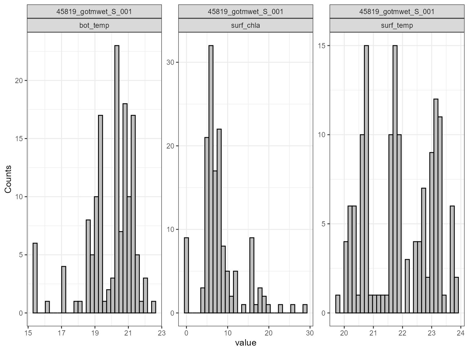

Scatter plot

The plot_scatter function plots the model output against the parameter value for each variable. This is useful for identifying relationships between the model output and the parameter value. For example, the plot below shows that there is a relationship between the model surface temperature (surf_temp_) and the parameter value of the scaling factor for shortwave radiation (MET_radswd), and also for surface chlorophyll-a (surf_chla) and the light extinction coefficient (light.Kw). When there is a low parameter value for Kw, the model chlorophyll-a is higher.

plot_scatter(sa_res)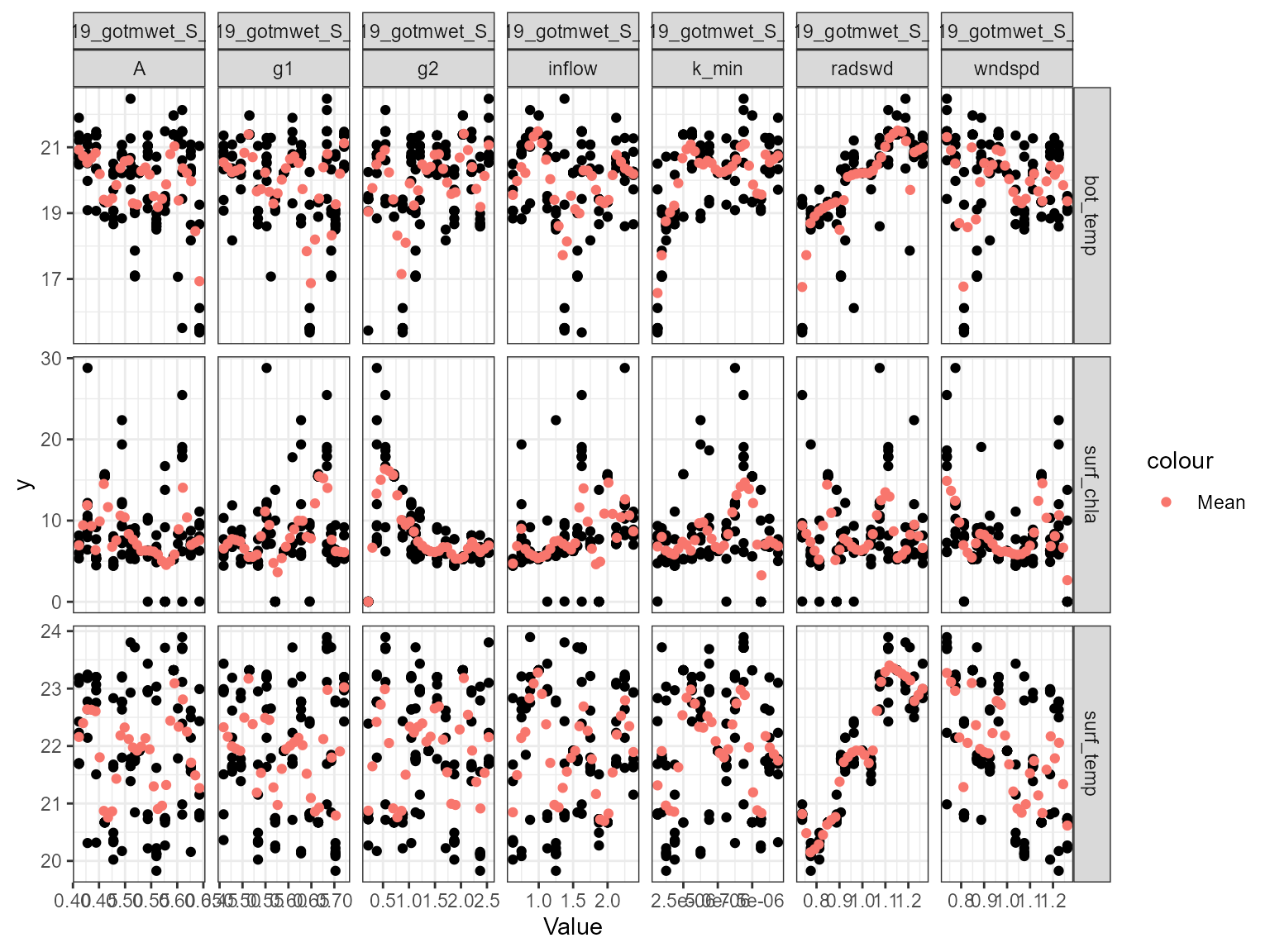

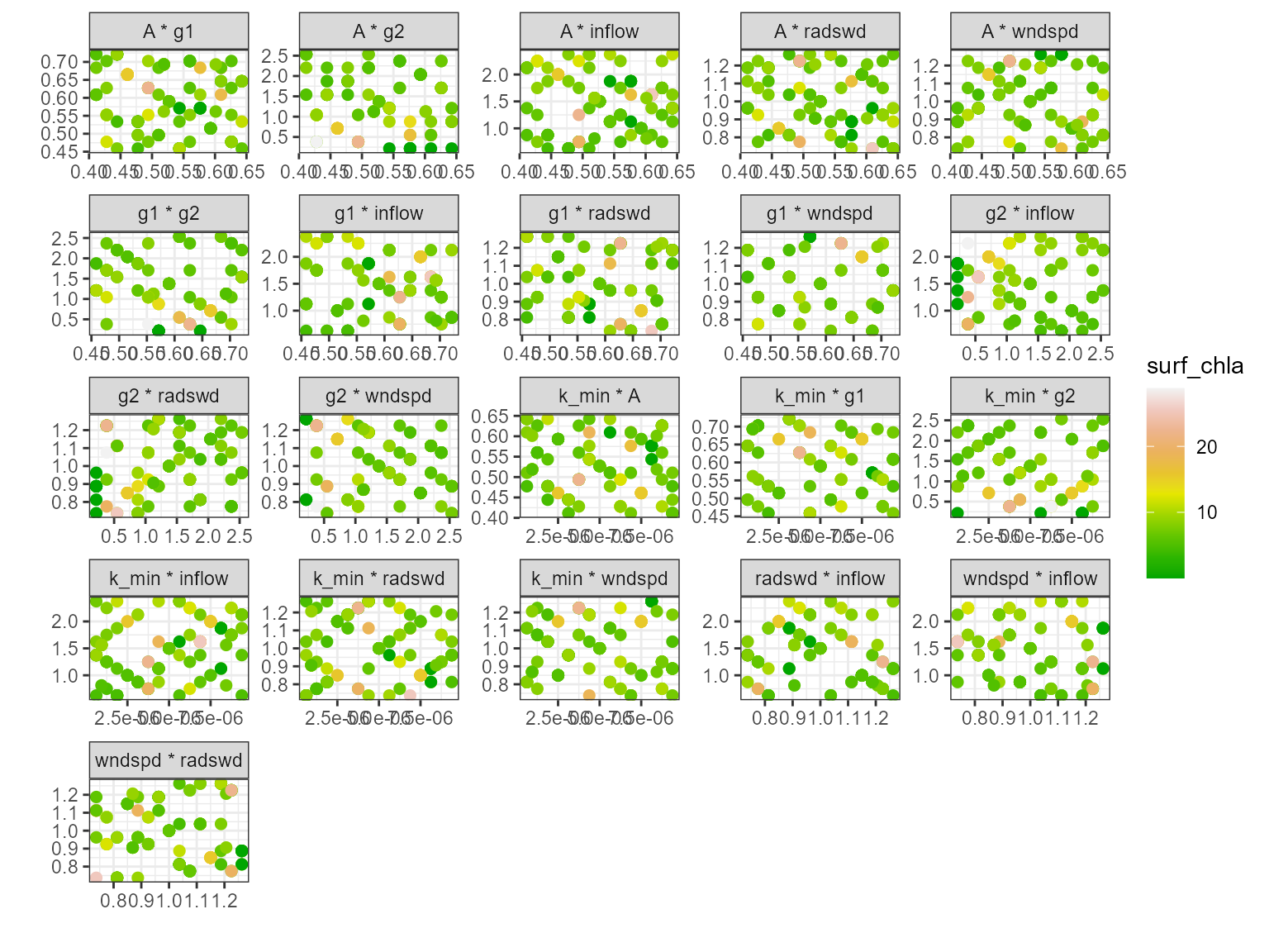
Multi-scatter plot

The plot_multiscatter function plots the parameters against each other for each variable. The parameter on top is the x-axis and the parameter below is the y-axis. This is useful for identifying relationships between the parameters and response variable.

pl <- plot_multiscatter(sa_res)

pl[[1]][1]
#> $surf_temp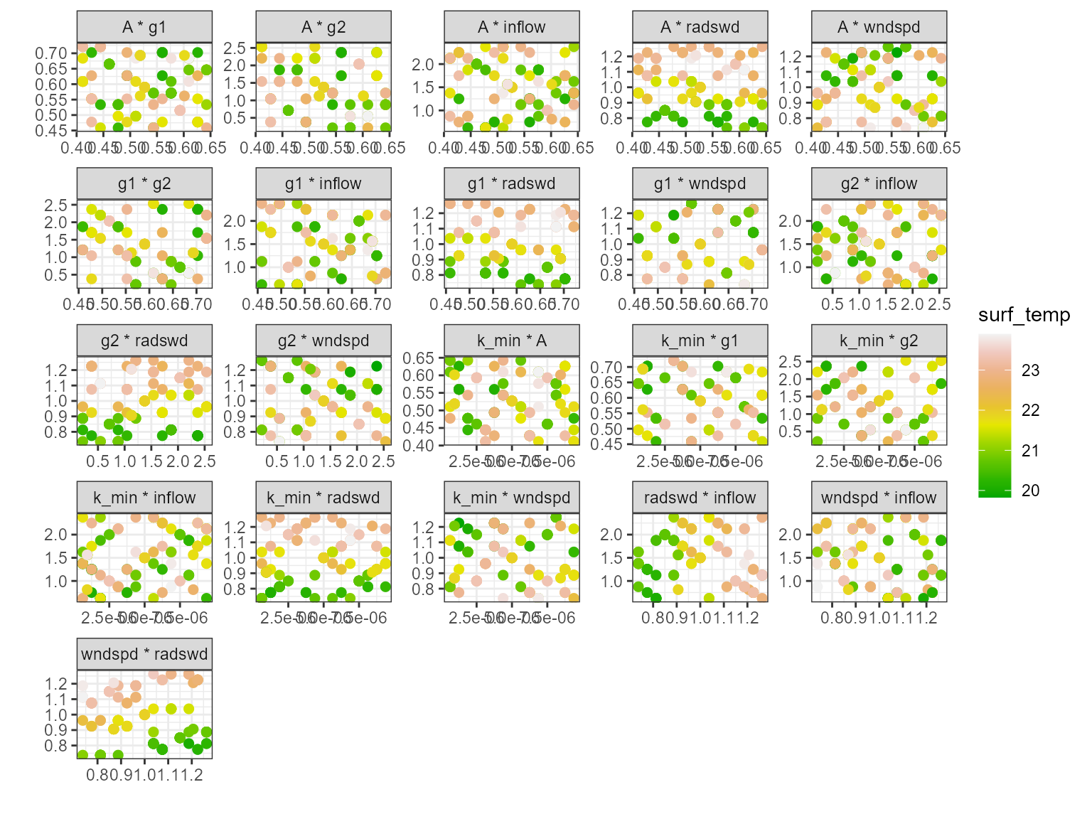

pl[[1]][2]
#> $bot_temp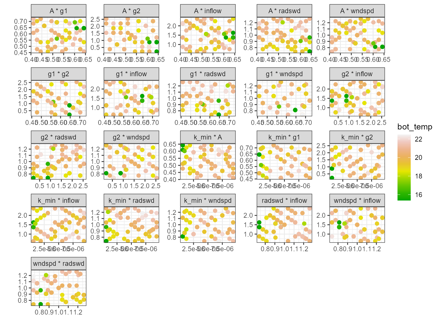

pl[[1]][3]
#> $surf_chla