Getting started
getting-started.RmdSetting up the Aquatic Ecosystem Model Ensemble is straight forward and can be done in a few steps. This vignette will guide you through the process of setting up the model for a lake in New Zealand.
library(AEME)
#>
#> Attaching package: 'AEME'
#> The following object is masked from 'package:stats':
#>
#>     time
library(sf) # For spatial data
#> Linking to GEOS 3.12.2, GDAL 3.9.3, PROJ 9.4.1; sf_use_s2() is TRUE
library(tmap) # For mapping
tmap_mode("view") # Set tmap mode to interactive view model
#> ℹ tmap mode set to "view".
tmap_options(basemap.server = "OpenStreetMap") # Set the basemap to OpenStreetMap
Lake data
The first step is to define the lake data. This includes the location of the lake, the depth and area of the lake, and the elevation of the lake.
# Define the location of the lake
lat <- -36.8898
lon <- 174.46898
# View the location of the lake in a map

coords <- data.frame(lat = lat, lon = lon) |>
  st_as_sf(coords = c("lon", "lat"), crs = 4326)

tm_shape(coords) +
  tm_bubbles() +
  tm_view(set_view = c(lon, lat, 16))
Depth and area data
The depth and area of the lake are required for the model. These can be obtained from a variety of sources, including regional councils, the New Zealand Hydrological Database, or from the lake owner.
# Set depth & area
depth <- 13.07 # Depth of the lake in metres
area <- 152343 # Area of the lake in m2
Elevation data
Elevation data can be acquired for New Zealand from the digital
elevation model hosted on the LINZ Data Service. There is a wrapper
function for this in the aemetools package. This requires
an API key from LINZ.
You can easily create a key on the LINZ website: https://data.linz.govt.nz/ or use the function within
the aemetools package to create one.
aemetools::create_linz_key()Then adding it to your .Renviron file.
# Add the LINZ API key to your .Renviron file
aemetools::add_linz_key(key = "your_key_here")
The get_dem_value function will return the elevation of
the lake in metres above sea level.
# Get the elevation of the lake
key <- Sys.getenv("LINZ_KEY")
elevation <- aemetools::get_dem_value(lat = lat, lon = lon, key = key)
elevation # in metres above sea level
#> [1] 29
elevation
#> [1] 29
We will now create a list of the lake data. This will be used to construct the AEME object.
# Define lake list
lake = list(
    name = "Wainamu",
    id = 45819,
    latitude = lat,
    longitude = lon,
    elevation = elevation,
    depth = depth,
    area = area
  )
Time data
The time data is required for the model. This includes the start and stop times for the model run.
# Define start and stop times
start <- "2020-08-01 00:00:00"
stop <- "2021-06-30 00:00:00"

time <- list(
    start = start,
    stop = stop
  )
Input data
Meteorological data
Download ERA5 data
We will use the aemetools package to download the ERA5
meteorological data for the location of our lake. This only works for
locations in New Zealand.
# Get ERA5 meteorological data
met <- aemetools::get_era5_point(lat = lat, lon = lon, years = 2020:2021)
View the summary of the meteorological data. The units have been converted to more common units used in aquatic ecosystem modelling.
# Summary of meteorological data
summary(met)
#>       Date              MET_tmpair       MET_tmpdew       MET_wnduvu
#>  Min.   :2020-01-01   Min.   : 9.137   Min.   : 3.094   Min.   :-10.826
#>  1st Qu.:2020-07-01   1st Qu.:13.406   1st Qu.: 9.326   1st Qu.: -2.087
#>  Median :2020-12-31   Median :15.801   Median :11.932   Median :  1.425
#>  Mean   :2020-12-31   Mean   :15.868   Mean   :11.835   Mean   :  1.128
#>  3rd Qu.:2021-07-01   3rd Qu.:18.327   3rd Qu.:14.488   3rd Qu.:  4.256
#>  Max.   :2021-12-31   Max.   :21.985   Max.   :19.221   Max.   : 10.963
#>    MET_wnduvv         MET_pprain        MET_ppsnow          MET_prsttn
#>  Min.   :-10.1534   Min.   : 0.0000   Min.   :0.000e+00   Min.   : 98312
#>  1st Qu.: -2.2161   1st Qu.: 0.1230   1st Qu.:0.000e+00   1st Qu.:100537
#>  Median :  0.8029   Median : 0.9502   Median :0.000e+00   Median :101066
#>  Mean   :  0.5009   Mean   : 4.2050   Mean   :4.553e-16   Mean   :101004
#>  3rd Qu.:  3.4222   3rd Qu.: 4.7504   3rd Qu.:2.168e-16   3rd Qu.:101481
#>  Max.   :  9.2317   Max.   :51.6713   Max.   :3.470e-15   Max.   :102963
#>    MET_radswd
#>  Min.   : 13.58
#>  1st Qu.:110.94
#>  Median :173.46
#>  Mean   :187.14
#>  3rd Qu.:262.12
#>  Max.   :530.52
The depth of this lake is 13.07 m, the area is 152343 m2, and the light extinction coefficient (Kw) is 1.31 m-1.
# Set Kw
Kw <- 1.31 # Light extinction coefficient in m-1
Hypsograph data
If you have hypsograph data for the lake, you can use it as input for the model. This is a critical input for the model, as it defines the relationship between the lake area and the lake elevation.
However, if you do not have hypsograph data, the model will use a simple cone-shaped hypsograph based on the lake depth and area. This is not ideal, but it will work for this example.
Required column names for the hypsograph data are area,
elev, and depth.
# Generate a simple hypsograph
hypsograph_simple <- data.frame(area = c(area, 0),
                         elev = c(elevation, elevation - depth),
                         depth = c(0, -depth))
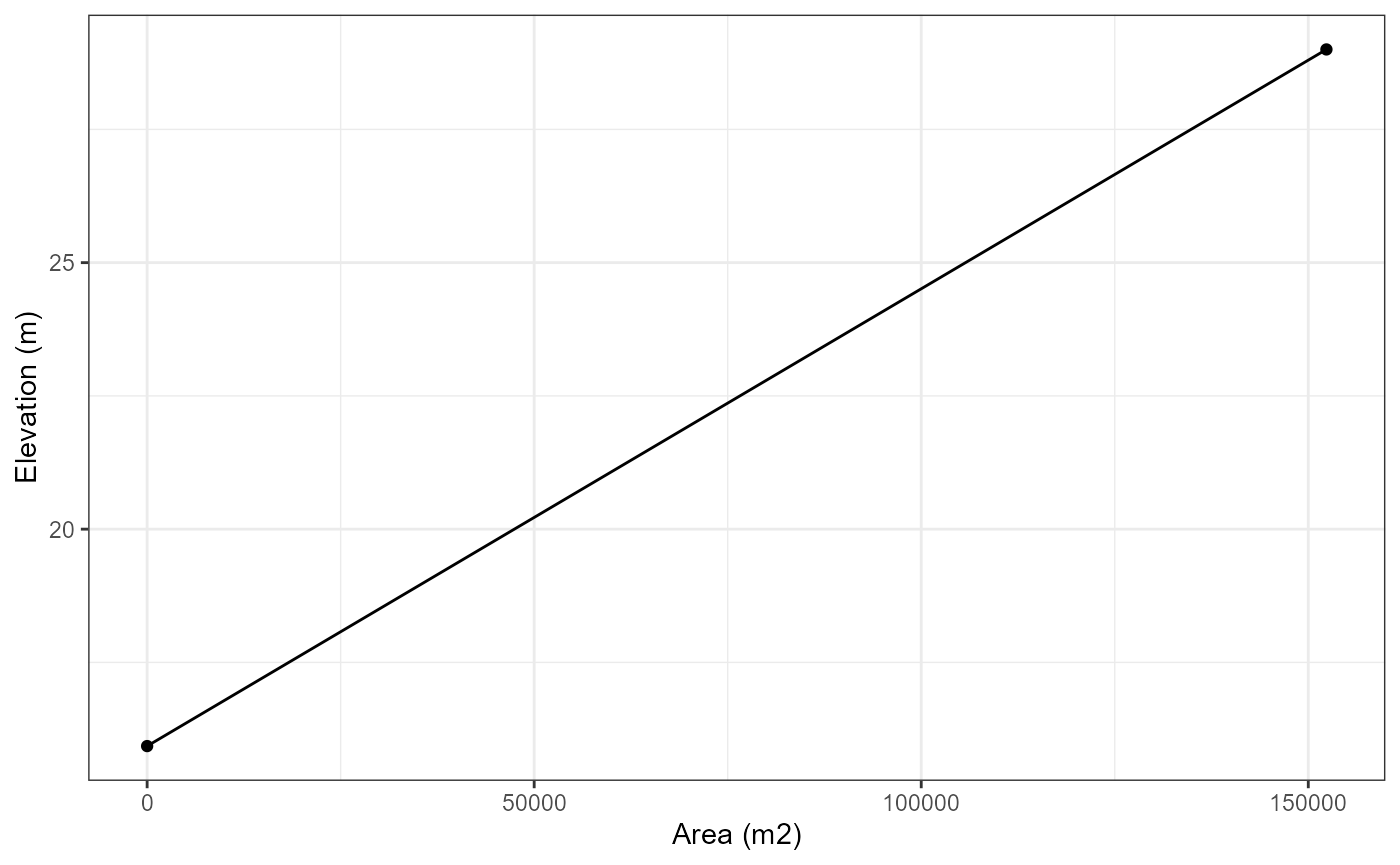
hypsograph_simple
#>     area  elev  depth
#> 1 152343 29.00   0.00
#> 2      0 15.93 -13.07
# Plot the hypsograph
library(ggplot2)

ggplot(hypsograph_simple, aes(x = area, y = elev)) +
  geom_line() +
  geom_point() +
  xlab("Area (m2)") +
  ylab("Elevation (m)") +
  theme_bw()
As you can see, the hypsograph is a simple cone shape. Ideally, you would have more detailed hypsograph data for your lake.
If you have information regarding the maximum depth of the lake, the
surface area and an estimate of volume development, you can generate a
hypsograph using the generate_hypsograph function. The
volume_development parameter is a scaling factor for the
volume development of the lake. Values below 1.5 are lakes with a
concave hypsograph, values above 1.5 are lakes with a convex hypsograph,
and values of 1.5 are lakes with a linear hypsograph.
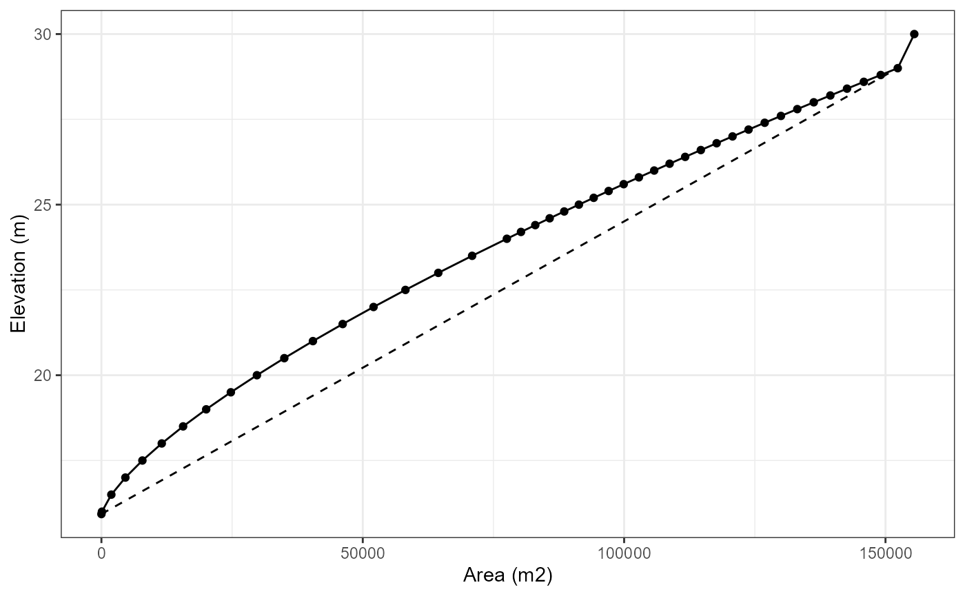
For Wainamu Lake, we will use a volume development of 1.62 which was calculated from a bathymetry survey of the lake. You can view this on the LERNZmp platform.
# Generate a hypsograph
hypsograph <- generate_hypsograph(max_depth = depth, surface_area = area,
                                  volume_development = 0.5, elev = elevation,
                                  ext_elev = 1)

ggplot(hypsograph, aes(x = area, y = elev)) +
  geom_line() +
  geom_point() +
  geom_line(data = hypsograph_simple, aes(x = area, y = elev),
            linetype = "dashed") +
  xlab("Area (m2)") +
  ylab("Elevation (m)") +
  theme_bw()
# Define input list
input = list(
    init_depth = depth,
    hypsograph = hypsograph,
    meteo = met,
    use_lw = TRUE,
    Kw = Kw
  )
Construct the AEME object
The aeme_constructor function will take the input data
and construct the AEME object. The minimum inputs are the
lake, time, and input data.
# Construct AEME object
aeme <- aeme_constructor(lake = lake,
                         time = time,
                         input = input)
#> Time step missing. Setting time step to 3600 seconds.
#> Spin up for models missing. Setting spin up to 2 for all models.
View AEME object
The AEME object can be inspected by printing it to the console. This will show the inputs that have been use to construct the object along with default values for inputs not provided.
aeme
#>             AEME
#> -------------------------------------------------------------------
#>   Lake
#> Wainamu (ID: 45819); Lat: -36.89; Lon: 174.47; Elev: 29m; Depth: 13.07m;
#> Area: 152343 m2; Shape file: Absent
#> -------------------------------------------------------------------
#>   Time
#> Start: 2020-08-01; Stop: 2021-06-30; Time step: 3600
#>  Spin up (days): GLM: 2; GOTM: 2; DYRESM: 2
#> -------------------------------------------------------------------
#>   Configuration
#>     Model controls: Absent
#>           Physical   |   Biogeochemical
#> DY-CD    : Absent     |   Absent
#> GLM-AED  : Absent     |   Absent
#> GOTM-WET : Absent     |   Absent
#> -------------------------------------------------------------------
#>   Observations
#> Lake: Absent; Level: Absent
#> -------------------------------------------------------------------
#>   Input
#> Inital profile: Absent; Inital depth: 13.07m; Hypsograph: Present (n=44);
#> Meteo: Present; Use longwave: TRUE; Kw: 1.31
#> -------------------------------------------------------------------
#>   Inflows
#> Data: Absent; Scaling factors: DY-CD: 1; GLM-AED: 1; GOTM-WET: 1
#> -------------------------------------------------------------------
#>   Outflows
#> Data: Absent; Scaling factors: DY-CD: 1; GLM-AED: 1; GOTM-WET: 1
#> -------------------------------------------------------------------
#>   Water balance
#> Method: 2; Use: obs; Modelled: Absent; Water balance: Absent
#> -------------------------------------------------------------------
#>   Parameters:
#> Number of parameters: 0
#> -------------------------------------------------------------------
#>   Output:
#> Number of ensembles: 0
#> DY-CD:
#> GLM-AED:
#> GOTM-WET:
In the configuration section of the output, under “Physical” and “Biogeochemical” for each model are labelle “Absent”. This is because the model configurations have not been built. This is done in the next step.
Building the AEME ensemble
Model controls
The model controls are the settings for the AEME ensemble. These are
read in from a CSV file. The default CSV file is stored within the
package and can be accessed using the get_model_controls
function. It has the argument use_bgc which is a logical
value to indicate whether to simulate the default biogeochemical
variables with the hydrodynamic variables or just the hydrodynamic
variables.
The model controls has the following columns:
-
var_aeme: The variable name in the AEME object -
simulate: Whether to simulate the variable -
inf_default: The default inflow value -
initial_wc: The initial water column value -
initial_sed: The initial sediment value
# Get model controls
model_controls <- get_model_controls()
model_controls
#>       var_aeme simulate inf_default initial_wc initial_sed conversion_aed
#> 1     HYD_flow    FALSE          NA         NA          NA     1.00000000
#> 2     HYD_temp     TRUE       15.00     11.000          NA     1.00000000
#> 3     HYD_dens    FALSE          NA         NA          NA     1.00000000
#> 4      RAD_par    FALSE          NA         NA          NA     1.00000000
#> 5     RAD_extc    FALSE          NA         NA          NA     1.00000000
#> 6   RAD_secchi    FALSE          NA         NA          NA     1.00000000
#> 7     CHM_salt     TRUE        0.00      0.000       0e+00     1.00000000
#> 8      CHM_oxy     TRUE       10.00     10.000       1e+01     0.03200000
#> 9      PHS_frp    FALSE        0.00      0.010       1e+06     0.03097376
#> 10     PHS_dop    FALSE        0.00      0.010       1e+06     0.03097376
#> 11    PHS_dopr    FALSE        0.00         NA          NA     0.03097376
#> 12     PHS_pop    FALSE        0.00      0.010       1e-04     0.03097376
#> 13    PHS_popr    FALSE        0.00         NA          NA     0.03097376
#> 14     PHS_pip    FALSE        0.00      0.002       5e-03     0.03097376
#> 15      PHS_tp    FALSE          NA         NA          NA     0.03097376
#> 16     NIT_amm    FALSE        0.05      0.020       1e+06     0.01400670
#> 17     NIT_nit    FALSE        0.20      0.015       1e+06     0.01400670
#> 18     NIT_don    FALSE        0.00      0.300       1e+06     0.01400670
#> 19    NIT_donr    FALSE        0.00         NA          NA     0.01400670
#> 20     NIT_pon    FALSE        0.00      0.100       1e-03     0.01400670
#> 21    NIT_ponr    FALSE        0.00         NA          NA     0.01400670
#> 22     NIT_pin    FALSE          NA      0.010       1e-03     0.01400670
#> 23      NIT_tn    FALSE          NA         NA          NA     0.01400670
#> 24     CAR_dic    FALSE       10.00      2.000       1e+06     0.01201100
#> 25     CAR_doc    FALSE        0.00      0.500       1e+06     0.01201100
#> 26    CAR_docr    FALSE        0.00         NA       1e+06     0.01201100
#> 27     CAR_poc    FALSE        0.00      0.200       1e-01     0.01201100
#> 28    CAR_pocr    FALSE        0.00         NA          NA     0.01201100
#> 29      CAR_ph    FALSE        0.00         NA          NA     1.00000000
#> 30     CAR_ch4    FALSE          NA         NA          NA     1.00000000
#> 31     SIL_rsi    FALSE        0.00      1.000       1e+07     1.00000000
#> 32     BAC_bac    FALSE        0.00         NA          NA     1.00000000
#> 33   PHY_dinof    FALSE        0.10      1.000       0e+00     1.00000000
#> 34   PHY_cyano    FALSE        0.10      1.000       0e+00     1.00000000
#> 35   PHY_nodul    FALSE        0.10      1.000       0e+00     1.00000000
#> 36   PHY_green    FALSE        0.10      1.000       0e+00     1.00000000
#> 37   PHY_crypt    FALSE        0.10      1.000       0e+00     1.00000000
#> 38   PHY_mdiat    FALSE        0.10      1.000       0e+00     1.00000000
#> 39  PHY_diatom    FALSE        0.10      1.000       0e+00     1.00000000
#> 40   PHY_tchla    FALSE          NA         NA          NA     1.00000000
#> 41     NCS_ss1    FALSE        5.00      3.000       3e-01     1.00000000
#> 42     NCS_ss2    FALSE        5.00      3.000       3e-01     1.00000000
#> 43     NCS_ss3    FALSE        5.00         NA          NA     1.00000000
#> 44     NCS_ss4    FALSE        5.00         NA          NA     1.00000000
#> 45     NCS_ss5    FALSE        5.00         NA          NA     1.00000000
#> 46     NCS_ss6    FALSE        5.00         NA          NA     1.00000000
#> 47     NCS_iss    FALSE          NA         NA          NA     1.00000000
#> 48     NCS_tss    FALSE          NA         NA          NA     1.00000000
#> 49    ZOO_zoo1    FALSE        0.10      1.000       0e+00     1.00000000
#> 50    ZOO_zoo2    FALSE        0.10         NA          NA     1.00000000
#> 51    ZOO_zoo3    FALSE        0.10         NA          NA     1.00000000
#> 52    ZOO_zoo4    FALSE        0.10         NA          NA     1.00000000
#> 53    ZOO_zoo5    FALSE        0.10         NA          NA     1.00000000
#> 54   FSH_fish1    FALSE        0.00      1.000          NA     1.00000000
#> 55   FSH_fish2    FALSE        0.00         NA          NA     1.00000000
#> 56   FSH_fish3    FALSE        0.00         NA          NA     1.00000000
#> 57   FSH_jelly    FALSE        0.00         NA          NA     1.00000000
#> 58 MAC_macalg1    FALSE        0.00         NA          NA     1.00000000
#> 59 MAC_macalg2    FALSE        0.00         NA          NA     1.00000000
#> 60 MAC_macalg3    FALSE        0.00         NA          NA     1.00000000
#> 61 MAC_macalg4    FALSE        0.00         NA          NA     1.00000000
#> 62   CLM_clam1    FALSE        0.00         NA          NA     1.00000000
#> 63   CLM_clam2    FALSE        0.00         NA          NA     1.00000000
#> 64   CLM_clam3    FALSE        0.00         NA          NA     1.00000000
#> 65     TRC_col    FALSE        0.00      0.000       0e+00     1.00000000
Build the ensemble
The build_aeme function will take the AEME object and
the model controls and build the ensemble. The model
argument is a character vector of the models to include in the ensemble.
The models available are dy_cd, glm_aed, and
gotm_wet.
# Select models
model <- c("dy_cd", "glm_aed", "gotm_wet")
# Path for model directory
path <- "aeme"

# Build ensemble
aeme <- build_aeme(aeme = aeme, model = model, model_controls = model_controls,
                   use_bgc = F, path = path)
#> Building simulation for Wainamu [2025-02-13 03:16:49]
#> No water level present. Using constant water level.
#> Estimating temperature using Stefan & Preud'homme (2007)...
#> Correcting water balance using estimated outflows (method = 2).
#> Calculating lake level using lake depth and a sinisoidal function.
#> Warning in dir.create(lake_dir, showWarnings = TRUE): cannot create dir
#> 'aeme\45819_wainamu', reason 'No such file or directory'
#> Building DYRESM-CAEDYM for lake wainamu
#> Copied in DYRESM par file
#> Writing DYRESM configuration
#> Writing DYRESM control file
#> Building GLM3-AED2 model for lake wainamu
#> Copied in GLM nml file
#> Building GOTM-WET for lake wainamu
#> Copied all GOTM configuration files

print(aeme)
#>             AEME
#> -------------------------------------------------------------------
#>   Lake
#> Wainamu (ID: 45819); Lat: -36.89; Lon: 174.47; Elev: 29m; Depth: 13.07m;
#> Area: 152343 m2; Shape file: Absent
#> -------------------------------------------------------------------
#>   Time
#> Start: 2020-08-01; Stop: 2021-06-30; Time step: 3600
#>  Spin up (days): GLM: 2; GOTM: 2; DYRESM: 2
#> -------------------------------------------------------------------
#>   Configuration
#>     Model controls: Present
#>           Physical   |   Biogeochemical
#> DY-CD    : Present    |   Absent
#> GLM-AED  : Present    |   Absent
#> GOTM-WET : Present    |   Absent
#> -------------------------------------------------------------------
#>   Observations
#> Lake: Absent; Level: Absent
#> -------------------------------------------------------------------
#>   Input
#> Inital profile: Present; Inital depth: 13.07m; Hypsograph: Present (n=44);
#> Meteo: Present; Use longwave: TRUE; Kw: 1.31
#> -------------------------------------------------------------------
#>   Inflows
#> Data: Absent; Scaling factors: DY-CD: 1; GLM-AED: 1; GOTM-WET: 1
#> -------------------------------------------------------------------
#>   Outflows
#> Data: Present; Scaling factors: DY-CD: 1; GLM-AED: 1; GOTM-WET: 1
#> -------------------------------------------------------------------
#>   Water balance
#> Method: 2; Use: obs; Modelled: Absent; Water balance: Present
#> -------------------------------------------------------------------
#>   Parameters:
#> Number of parameters: 0
#> -------------------------------------------------------------------
#>   Output:
#> Number of ensembles: 0
#> DY-CD:
#> GLM-AED:
#> GOTM-WET:
By default, the build_aeme function will build the file
configuration for each model. This will create the necessary files for
each model to run. The files are also stored in the aeme
object in the configuration slot with a list for
hydrodynamic and ecosystem model configurations.
# View the files
cfg <- configuration(aeme)
names(cfg[["glm_aed"]])
#> [1] "hydrodynamic" "ecosystem"
All of the information and data needed to run an ensemble of models
is now contained within the aeme object. This allows for
easy storage of all the data and also for easy sharing of the data with
others. Sharing the aeme object with others allows them to
run the ensemble of models without needing to reconstruct the
object.
# Run the ensemble
aeme <- run_aeme(aeme = aeme, model = model, path = path)
#> Running models... (Have you tried parallelizing?) [2025-02-13 03:16:51]
#> DYRESM-CAEDYM running... [2025-02-13 03:16:51]
#> DYRESM-CAEDYM run successful! [2025-02-13 03:17:10]
#> GLM-AED running... [2025-02-13 03:17:10]
#> GLM-AED run successful! [2025-02-13 03:17:11]
#> GOTM-WET running... [2025-02-13 03:17:11]
#> GOTM-WET run successful! [2025-02-13 03:17:11]
#> Model run complete![2025-02-13 03:17:11]
#> Retrieving and formatting dyresmTEMPTURE_Var for model dy_cd
#> Retrieving and formatting dyresmSALINITY_Var for model dy_cd
#> Retrieving and formatting temp for model glm_aed
#> Retrieving and formatting salt for model glm_aed
#> Retrieving and formatting temp for model gotm_wet
#> Retrieving and formatting salt for model gotm_wet
View the output
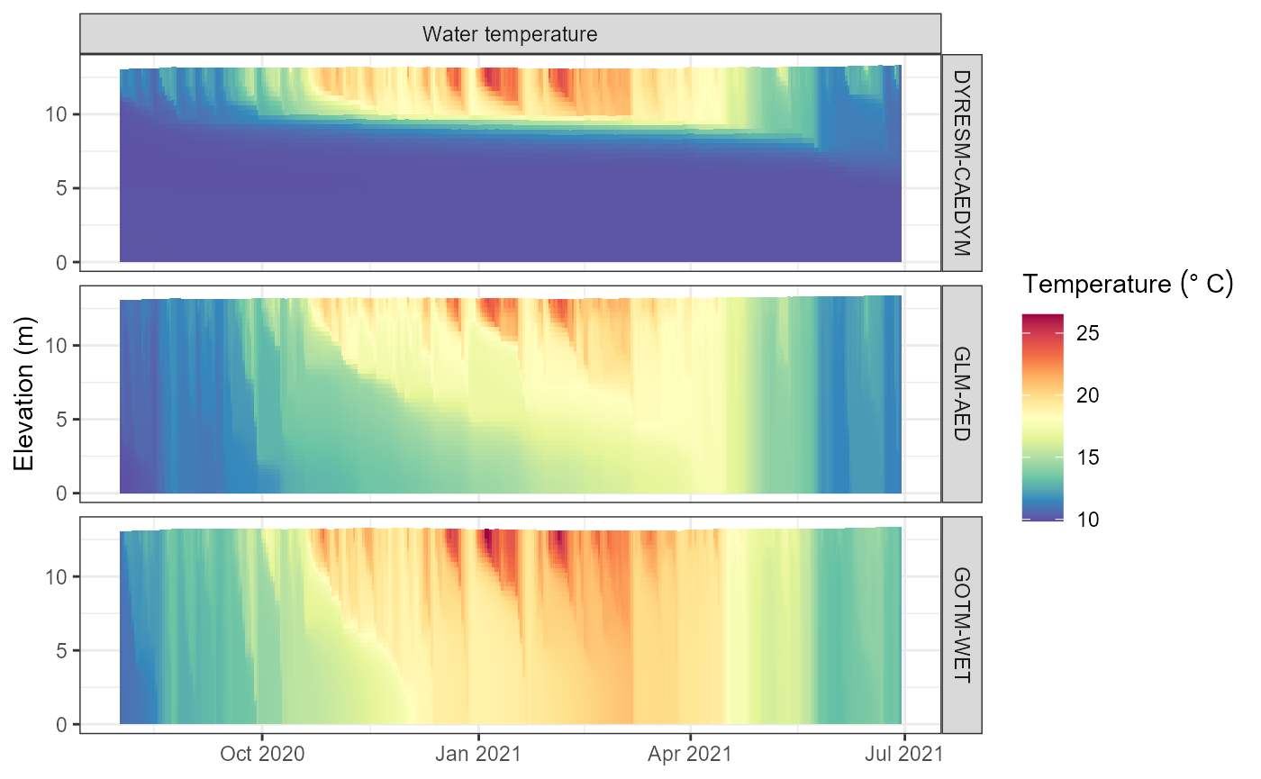
The output from the model run is stored in the output
slot of the aeme object. This is a list with a list for
each model. The list contains the output data from the model run.
# View the output
plot_output(aeme = aeme, model = model)
#> Warning: Removed 246 rows containing missing values or values outside the scale range
#> (`geom_col()`).
Saving the AEME object
Saving the aeme object to a file can be done using the
saveRDS function. This will save the object to a file with
the .rds.
# Save the AEME object
saveRDS(aeme, "aeme.rds")