Introduction to AEME • AEME

Summary

The AEME package hosts three one-dimensional hydrodynamic models: the DYnamic REservoir Simulation Model (DYRESM), the General Lake Model (GLM), and the General Ocean Turbulence Model (GOTM, which has been adapted for closed basins for application to lakes and reservoirs). The models can be coupled to their corresponding water quality models, the DYRESM-CAEDYM (Computational Aquatic Ecosystem Dynamics Model), GLM-AED2 (Aquatic Ecosystem Dynamics Model 2), and GOTM-WET (Water Ecosystem Tool).

Key aspects of the AEME package include:

Defined S4 class for aeme objects
Configuration of models from common and standardised inputs
Standardised calibration, manipulation and visualisation

AEME object

Description

The aeme object is the main object in the AEME package. It is an S4 class that contains all the information required to run a model. The aeme object contains the following slots:

lake - a list object containing information about the lake (name, id, latitude, longitude, elevation, depth, area)
time - a list object containing information about the time (start, stop, spin_up, time_step)
configuration - a list object containing information about the configuration (model_controls, dy_cd, glm_aed, gotm_wet)
observations - a list object containing information about the observations (lake, level)
inputs - a list object containing information about the inputs (init_profile, init_depth, hypsograph, meteo, use_lw, Kw)
inflows - a list object containing information about the inflows (data, factor)
outflows - a list object containing information about the outflows (data, outflow_lvl, factor)
water_balance - a list object containing information about the water balance configuration (use, method, data)
parameters - a data.frame describing the parameters to be input with column names (model, file, name, value, min, max, module, group)
output - a list object containing information about the outputs (n_members)

Lake

The lake slot contains information about the lake. It is a list object that contains the following objects:

name - Name of the lake (character).
id - Lake ID (character or numeric).
latitude - Latitude of the lake (numeric). If not provided, the latitude will be calculated from the centroid of the shape.
longitude - Longitude of the lake (numeric). If not provided, the longitude will be calculated from the centroid of the shape.
elevation - Elevation of the lake (numeric).
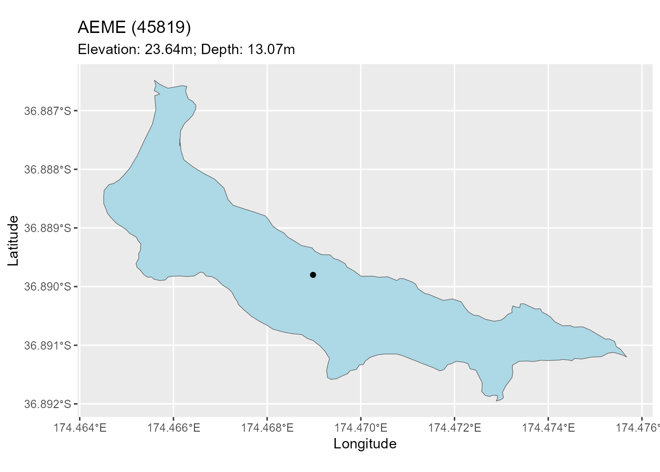
shape - Shape of the lake (sf object). The shape of the lake can be represented as a polygon. The centroid of the polygon will be used to calculate the latitude and longitude of the lake.
depth - Max depth of the lake (m) (numeric). Depth and area are used to generate a simple hypsographic curve if none is provided in the inputs slot.
area - Surface area of the lake (m2) (numeric)

Objects in bold are required for building and running the model.

Time

The time slot contains information about the time. It is a list object that contains the following objects:

start - Start date of the simulation (character). The start date must be in the format YYYY-MM-DD HH:MM:SS.
end - End date of the simulation (character). The end date must be in the format YYYY-MM-DD HH:MM:SS.
timestep - Timestep of the simulation (numeric). The timestep must be in seconds.
spin_up - List of spin up periods of the simulation for each model (numeric). The spin up period must be in days. The spin up period is the period of time that the model is run before the simulation period. The spin up period is used to initialise the model which is then discarded when examining the simulation period.

Configuration

The configuration slot is a list that contains each of the model configurations. This includes the configurations files for the hydrodynamic components as well as the aquatic ecosystem model components:

Files for hydrodynamic and ecosystem models.
Model	Hyrodynamic	Ecosystem
DYRESM-CAEDYM	.cfg file and .par file	.con, caedym3p1.bio, caedym3p1.chm and caedym3p1.sed files
GLM-AED	glm3.nml file	aed2.nml, phytos.nml, zoops.nml files
GOTM-WET	gotm.yaml and output.yaml files	fabm.yaml file

When build_aeme() is ran, the model_controls data.frame that is passed to the function as an argument is added to the configuration slot.

For more details on the model_controls, see it’s section below.

Observations

The observations slot is a list that contains observations of in-lake (lake) variables (e.g. water temperature, chlorophyll-a, dissolved oxygen etc.) and water level (level). The observations are used to assess model performance using the function and also to calibrate the model using the aemetools package.

The lake observations are stored in a data frame with the following columns:

Date - Date of the observation (character). The date must be in the format YYYY-MM-DD HH:MM:SS.
depth - Depth of the observation (m) (numeric). The depth must be in metres.
var - Variable name of the observation (character). The variable names an input preparation are designed in the AEME inputs article.
value - Value of the observation (numeric).

The level observations are stored in a data frame with the following columns:

Date - Date of the observation (character). The date must be in the format YYYY-MM-DD HH:MM:SS.
value - Value of the observation (numeric).

Input

The input slot is a list that contains the following objects:

init_profile - profile to initialise the lake simulation (data.frame). It has the columns: “depth”, “temperature” and “salt”. If this is not provided, it is automatically generated using the values in the model_controls.
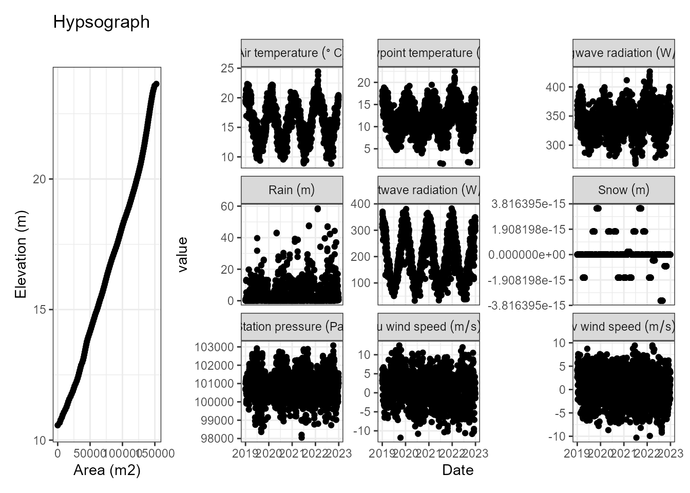
init_depth - depth of the lake when initialising the model (vector), If not provided, will assume the depth from the hypsograph.
hypsograph - the lake hypsograph. This is a data.frame with the columns “elev”, “depth” and “area”. If you do not have this data, you can generate one using the generate_hypsograph() function.
meteo - the meteorological data. A data.frame which at a minimum must contain the columns date (“Date”), air temperature (“MET_tmpair), wind speed (”MET_wndspd”) and shortwave radiation (“MET_radswd”). See AEME Inputs
use_lw - Logical switch to use longwave radiation. Defaults to TRUE.
Kw - the light extinction coefficient ( $m^{-1}$ ).

Inflows

The inflows slot is a list that contains the following objects:

data - named list of data.frames which contain the columns date (“Date”), flow (“HYD_flow”; $m^3 day^{-1}$ ). Temperature can also be provided (“HYD_temp”), however if not provided then it will be estimated using air temperature. The name for the list will be used as the stream identifier in each model. If method in the water_balance section is set to3, then “wbal” will be added to the data, this contains a separate inflow for each model, estimated using the different evaporation functions inside each model.
factor - list of scaling factors to be applied to the inflows. Named according to each model.

If no inflows are present then this slot will be empty.

Outflows

The outflows slot is a list that contains the following objects:

data - named list of data.frames which contain the columns date (“Date”), flow (“HYD_flow”; $m^3 day^{-1}$ ). If method in the water_balance section is set to 2 or 3, then “wbal” will be added to the data, this contains a separate outflow for each model, estimated using the different evaporation functions inside each model.
factor - list of scaling factors to be applied to the outflows. Named according to each model. However, this can also be passed as a parameter in the model_parameters section and calibrated there. This is the preferred method for applying scaling factors.

If no outflows are present then this slot will be empty.

Water balance

The water balance slot is generated internally when the build_aeme() function is called and the wb_method is set to 2 or 3. The slot contains:

use: define which lake level to use. Can either be observed (“obs”) or modelled (“mod”) lake level. Default = “obs”.
method: This can be 1 (no inflows or outflows) or 2 (outflows calculated) or 3 (inflows and outflows calculated). The default is 2 .
data: list of two data.frames. “wbal” which contains the diagnostics for estimating evaporation and water balance for each model and “model” which contains the modelled lake water level if use is “mod”.

Parameters

The parameters slot contains a data.frame of parameters which are used when building the model. These will update the default model parameters or scale the meteorological or scale the inflows and outflows for each model.

The columns for the parameters data.frame are:

model - Either “dy_cd”, “glm_aed” and “gotm_wet”.
file - Either the name of the file e.g. “glm3.nml” for model specific files or “met” for meteorological variables or “inf” for inflow or “wdr” for outflows. (Outflows were initiallly referred to as withdrawals, hence the “wdr” notation, this will probably be updated to reflect the current outflows slot soon…).
name - Name of the parameter. If the name of the parameter is nested in a nml/yaml file, then the whole hierarchy needs to be provide with each level separated by a “/” e.g. “light/Kw” for Kw in GLM-AED.
value - Value of the parameter.
min - Minimum range of the parameter. This is used in the aemetools::calib_aeme() and aemetools::sa_aeme() function.
max - Maximum range of the parameter. This is used in the aemetools::calib_aeme() and aemetools::sa_aeme() function.
module - Module that the parameter is in. Not necessary, but is helpful for identifying which parameters are in which module for GLM-AED and GOTM-WET.
group - Phytoplankton group. This is only used for GOTM-WET phytoplankton parameters.

There is a function get_aeme_parameters() which allows you to select parameters based on model and module. See ?get_aeme_parameters() for more details.

Output

The output slot is a list that is updated when run_aeme() is executed. Each time it is executed, variable outputs designated in the model_controls will be added to the Aeme object.

Model controls

The model_controls is a data.frame generated by the get_model_controls(). The data.frame has the columns:

var_aeme - character; the AEME variable name
simulate - logical; add the variable to the Aeme object
inf_default - numeric; default value to use in the inflows if none present in the inflows. This is particularly important for configuring water chemistry for the inflows if use_bgc = TRUE.
initial_wc - numeric; value to use in initialising the model. This will be automatically updated if the variable is present in the observations slot.
initial_sed - numeric; value to use in intialising the sediment module for the DYRESM-CAEDYM model.
conversion_aed - numeric; factor to multiply by to convert to GLM-AED units.

When the model is built the mode

Creation

The aeme object can be created using the aeme_constructor() function. It requires the basic inputs to from a YAML file using the yaml_to_aeme function. The YAML file contains all the information required to run the model.

# Define lake list
lat <- -36.88921
lon <- 174.4669
depth <- 13.08
area <- 153648

lake <- list(
    latitude = lat,
    longitude = lon,
    # elevation = elevation,
    depth = depth,
    area = area
  )
time <- list(
  start = as.POSIXct("2020-07-01"),
  stop = as.POSIXct("2022-06-30")
)

hypsograph <- generate_hypsograph(max_depth = depth, surface_area = area,
                                  volume_development = 1.2)

met <- aemetools::get_era5_point(lat = lat, lon = lon, years = 2020:2022)

#' Define input list
input = list(
  hypsograph = hypsograph,
  meteo = met,
  Kw = 1.21
)

aeme <- aeme_constructor(lake = lake, time = time, input = input)

slotNames(aeme)
#>  [1] "lake"          "time"          "configuration" "observations" 
#>  [5] "input"         "inflows"       "outflows"      "water_balance"
#>  [9] "output"        "parameters"

Manipulation

The aeme object can be manipulated using the AEME package functions. The functions are defined by the slot names of the aeme object. For example, the lake slot can be manipulated using the lake function.

# Load lake data
lke <- lake(aeme)
# Print lake data to console
print(lke)
#> $name
#> [1] "Wainamu"
#> 
#> $id
#> [1] "LID45819"
#> 
#> $latitude
#> [1] -36.88921
#> 
#> $longitude
#> [1] 174.4669
#> 
#> $elevation
#> [1] 23.2
#> 
#> $depth
#> [1] 13.48
#> 
#> $area
#> [1] 153648

# Change lake name
lke[["name"]] <- "AEME"

# reassign lake data to aeme object
lake(aeme) <- lke

aeme
#>             AEME 
#> -------------------------------------------------------------------
#>   Lake
#> AEME (ID: LID45819); Lat: -36.89; Lon: 174.47; Elev: 23.2m; Depth: 13.48m;
#> Area: 153648 m2
#> -------------------------------------------------------------------
#>   Time
#> Start: 2013-07-01; Stop: 2023-06-30; Time step: 3600
#>  Spin up (days): GLM: 1095; GOTM: 1095; DYRESM: 1095
#> -------------------------------------------------------------------
#>   Configuration
#>     Model controls: Present
#>           Physical   |   Biogeochemical
#> DY-CD    : Absent     |   Absent 
#> GLM-AED  : Present    |   Present
#> GOTM-WET : Present    |   Present
#> -------------------------------------------------------------------
#>   Observations
#> Lake: Present; Level: Absent
#> -------------------------------------------------------------------
#>   Input
#> Inital profile: Present; Inital depth: 13.48m; Hypsograph: Present (n=53);
#> Meteo: Present; Use longwave: TRUE; Kw: 1.214286
#> -------------------------------------------------------------------
#>   Inflows
#> Data: Present; Scaling factors: DY-CD: 1; GLM-AED: 1; GOTM-WET: 1
#> -------------------------------------------------------------------
#>   Outflows
#> Data: Present; Scaling factors: DY-CD: 1; GLM-AED: 1; GOTM-WET: 1
#> -------------------------------------------------------------------
#>   Water balance
#> Method: 2; Use: obs; Modelled: Absent; Water balance: Present
#> -------------------------------------------------------------------
#>   Parameters: 
#> Number of parameters: 18
#> -------------------------------------------------------------------
#>   Output: 
#> 
#> DY-CD:    
#> GLM-AED:  
#> GOTM-WET:

Visualisation

The aeme object can be visualised simply using the plot function. The plot function can be applied to the different slots of the aeme object. For example, the lake slot can be visualised using the plot function.

plot(aeme, "lake")

plot(aeme, "input")

Build Model Ensemble

model_controls <- get_model_controls()
inf_factor = c("dy_cd" = 1, "glm_aed" = 1, "gotm_wet" = 1)
outf_factor = c("dy_cd" = 1, "glm_aed" = 1, "gotm_wet" = 1)
model <- c("dy_cd", "glm_aed", "gotm_wet")
path <- "aeme"
aeme <- build_aeme(path = path, aeme = aeme, model = model,
                            model_controls = model_controls, inf_factor = inf_factor,
                            ext_elev = 5, use_bgc = TRUE)
#> Building simulation for AEME [2025-02-17 04:57:34]
#> Missing state variables in inflows: CHM_oxy
#> Added default values for missing variables.
#> Missing state variables in inflows: CHM_oxy
#> Added default values for missing variables.
#> Missing state variables in inflows: CHM_oxy
#> Added default values for missing variables.
#> Missing state variables in inflows: CHM_oxy
#> Added default values for missing variables.
#> Missing state variables in inflows: CHM_oxy
#> Added default values for missing variables.
#> Missing state variables in inflows: CHM_oxy
#> Added default values for missing variables.
#> No water level present. Using constant water level.
#> Correcting water balance using estimated outflows (method = 2).
#> Calculating lake level using lake depth and a sinisoidal function.
#> Warning in dir.create(lake_dir, showWarnings = TRUE): cannot create dir
#> 'aeme\LID45819_aeme', reason 'No such file or directory'
#> Building DYRESM-CAEDYM for lake aeme
#> Copied in DYRESM par file
#> Writing DYRESM configuration
#> [1] "TEMPTURE SALINITY DO"
#> Writing DYRESM control file
#> Building GLM3-AED2 model for lake aeme
#> Copied in GLM nml file
#> Copied in AED nml file
#>    oxy_initial   = 625 replaced with 312.5
#> Building GOTM-WET for lake aeme
#> Copied all GOTM configuration files
#> instances/abiotic_water/initialization/sO2W 13 replaced with 10
#> Warning in input_model_parameters(aeme = aeme, model = model, param = param, :
#> No parameters in 'param' for dy_cd.
aeme
#>             AEME 
#> -------------------------------------------------------------------
#>   Lake
#> AEME (ID: LID45819); Lat: -36.89; Lon: 174.47; Elev: 23.2m; Depth: 13.48m;
#> Area: 153648 m2
#> -------------------------------------------------------------------
#>   Time
#> Start: 2013-07-01; Stop: 2023-06-30; Time step: 3600
#>  Spin up (days): GLM: 1095; GOTM: 1095; DYRESM: 1095
#> -------------------------------------------------------------------
#>   Configuration
#>     Model controls: Present
#>           Physical   |   Biogeochemical
#> DY-CD    : Present    |   Present
#> GLM-AED  : Present    |   Present
#> GOTM-WET : Present    |   Present
#> -------------------------------------------------------------------
#>   Observations
#> Lake: Present; Level: Absent
#> -------------------------------------------------------------------
#>   Input
#> Inital profile: Present; Inital depth: 13.48m; Hypsograph: Present (n=54);
#> Meteo: Present; Use longwave: TRUE; Kw: 1.214286
#> -------------------------------------------------------------------
#>   Inflows
#> Data: Present; Scaling factors: DY-CD: 1; GLM-AED: 1; GOTM-WET: 1
#> -------------------------------------------------------------------
#>   Outflows
#> Data: Present; Scaling factors: DY-CD: 1; GLM-AED: 1; GOTM-WET: 1
#> -------------------------------------------------------------------
#>   Water balance
#> Method: 2; Use: obs; Modelled: Absent; Water balance: Present
#> -------------------------------------------------------------------
#>   Parameters: 
#> Number of parameters: 18
#> -------------------------------------------------------------------
#>   Output: 
#> 
#> DY-CD:    
#> GLM-AED:  
#> GOTM-WET:

cfg <- configuration(aeme)